Reproducing 'Does data interpolation contradict statistical optimality?'
Introduction
During one of my biweekly research meetings, my group reviewed Does data interpolation contradict statistical optimality? by Mikhail Belkin, Alexander Rakhlin, and Alexandre B, Tsybakov
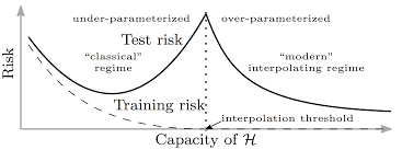
The aim of this paper was to show that interpolating training data can still lead to optimal results in nonparametric regression and prediction with square loss. Since the double descent phenomenon exhibits itself when the model capacity surpasses the “interpolation threshold”, I thought that reproducing the results from this paper would help me understand how a model interpolates data.
[1]
 )
)
Math and Code
import numpy as np
import os
import numpy.linalg as lin
import matplotlib.pyplot as plt
import scipy.stats as stats
This paper takes a look at interpolation using the Nadaraya-Watson Estimator.
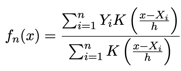
Let \((X, Y)\) be a random pair on \(\mathbb{R}^{d} \times \mathbb{R}\) with distribution \(P_{XY}\), and let \(\mathbb{E}[Y \vert X = x]\) be the regression function.
Given a sample \((X_{1}, Y_{1}),...,(X_{n}, Y_{n})\) drawn independently from \(P_{XY}\), we can approximate $f(x)$ using the Nadaraya-Watson Estimator where \(K: \mathbb{R}^{d} \rightarrow \mathbb{R}\) is a kernel function and \(h > 0\) is a bandwidth
def nadaraya_watson_estimator(x, X, Y, h, K=stats.norm.pdf):
    cols=[]
    for i in range(len(X)):

        cols.append(np.array(K((x - X[i])/h)))


    Kx = np.column_stack(tuple(cols))

    row_sums = np.sum(Kx, axis=1)

    W = Kx / row_sums[:, None]

    result = np.matmul(W,Y)
    result.shape = (result.shape[0], 1)
    return result
Note: Since we are dealing with singular kernels that approach infinity when their argument tends to zero, we will have to use a modified version
def singular_nadaraya_watson_estimator(x, X, Y, h, K=stats.norm.pdf, a=1):

    cols = []
    for i in range(len(X)):

        condition = False
        for boolean in [k==0 for k in x - X[i]]:
            if boolean:
                condition = True
                cols.append(np.array([Y[i]] * len(x)))
                break

        if condition == False:
            cols.append(np.array(K((x - X[i])/h, a)))


    Kx = np.column_stack(tuple(cols))

    row_sums = np.sum(Kx, axis=1)

    W = Kx / row_sums[:, None]

    result = np.matmul(W,Y)
    result.shape = (result.shape[0], 1)
    return result
The two singular kernels we will be focusing on are:
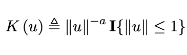
def sing_kernel_1(x,a):
    return 1/(abs(x))**a
and
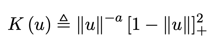
def sing_kernel_2(x, a):
    return (1/(abs(x))**a)*(1-abs(x))**2
The data generating functions we will look at are
def actual_regression_1(x):
    return 5*np.sin(x)
and
def binary_classification(x):
    outs = np.array([])

    for element in x:
        if abs(element) > .4:
            outs = np.append(outs, [1])
        else:
            outs = np.append(outs, [0])
    return outs
Some notes:
- Because of input size mismatches, I used
abs()instead oflinalg.norm()since I pass in the elements as arrays, but they are really (x, y) which are both just 1 dimensional real numbers - The indicator function on
sing_kernel_1gave me errors when I tried implementing it, so i removed it. The kernel’s singularity as the argument goes to infinity is still present. - The data from the sinusoidal function (p.4 of the paper) does not seem to be randomly sampled, so I did not randomly sample it either
Results
Sine curve with singular_kernel_1:
The estimator fits the curve fairly well for values of a > .8. For some reason, the bandwidth, h, doesn’t do anything to this specific example. Because the best value of h in the paper was .4, I chose to keep h constant.
Sine curve with standard Gaussian kernel:
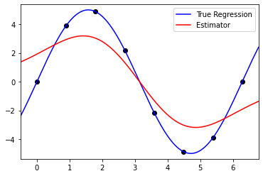
There are no animations for different parameters because the only tunable parameter is the bandwidth, h, which was held constant at .4
Code (from notebook)
#np.random.seed(100)
n = 8
#epsilon = np.random.normal(loc = 0, scale = 2, size = n)
X = np.linspace(0, 2*np.pi, n)
#np.random.normal(loc = 0, scale = 3, size=n)
Y = actual_distribution_1(X)
x_axis = np.linspace(-1, 7, 100000)
# Singular Kernel
h=.4
a=1.5

plt.scatter(X, Y, color='k')
plt.plot(x_axis, actual_distribution_1(x_axis), 'b-')
plt.plot(x_axis, singular_nadaraya_watson_estimator(x_axis, X, Y, h, K=sing_kernel_1,a=a), 'r-')
plt.xlim(min(X) - .5, max(X) + .5)
plt.ylim(min(Y) - .5, max(Y) + .5)
plt.legend(['True Regression', 'Estimator'])
plt.show()
# Non-singular Kernel

h=n**(-1/(2*0 + len(x_axis)))
plt.scatter(X, Y, color='k')
plt.plot(x_axis, actual_distribution_1(x_axis), 'b-')
plt.plot(x_axis, nadaraya_watson_estimator(x_axis, X, Y, h), 'r-')
plt.xlim(min(X) - .5, max(X) + .5)
plt.ylim(min(Y) - .5, max(Y) + .5)
plt.legend(['True Regression', 'Estimator'])
plt.show()
Binary Data with singular_kernel_2:
In this animation, I sweep through several values for h with a constant. Then I hold h constant and sweep through several values of a
Binary data with standard Gaussian kernel
The only tunable parameter here is h
Code (from notebook)
#np.random.seed(100)
n = 8
#epsilon = np.random.normal(loc = 0, scale = 2, size = n)
X = np.random.choice(np.linspace(-1, 1, 20), n)
Y = binary_distribution(X)
x_axis = np.linspace(-1, 1, 500)
h=n**(-1/(2*0 + len(x_axis)))
a=1
plt.scatter(X, Y, color='k')
plt.plot(x_axis, np.array([.5] * len(x_axis)), 'b--')
plt.plot(x_axis, singular_nadaraya_watson_estimator(x_axis, X, Y, h, K=sing_kernel_2, a=a), 'r-')
plt.xlim(min(X) -.1, max(X) + .1)
plt.ylim(min(Y) - .1, max(Y) + .1)
plt.title('a = {:.2f}; h = {:.2f}'.format(a, h), fontsize=12)
plt.legend(['Boundary', 'Estimator'])
plt.show()
h =.4
plt.scatter(X, Y, color='k')
plt.plot(x_axis, np.array([.5] * len(x_axis)), 'b--')
plt.plot(x_axis, nadaraya_watson_estimator(x_axis, X, Y, h), 'r-')
plt.xlim(min(X) - .1, max(X) + .1)
plt.ylim(min(Y) - .1, max(Y) + .1)
plt.title('h = {:.2f}'.format(h))
plt.legend(['Boundary', 'Estimator'])
plt.show()
Conclusion
After reproducing these results, I emailed Mikhail Belkin to get his thoughts on the connection between this paper and a previous paper he wrote on the double descent phenomenon. His reply was very similar to what my group thought the connection may be: interpolation is consistent with the current practice of deep learning. The most important thing to realize is that there is still not a proven, complete connection between modern machine learning methods and the model shown in this post.
References:
- Does data interpolation contradict statistical optimality? - https://arxiv.org/abs/1806.09471
- [1] - https://www.cs.ubc.ca/labs/lci/mlrg/slides/dl_generalization.pdf