Double Descent Testbed
The Double Descent Phenomenon
Modern machine learning models, such as deep neural networks, have given us the ability to observe how models with immense hypothesis classes (i.e. the set of functions that are learnable by the mode) are able to perform on complex, high dimensional data sets. Based on what we know about the bias-variance tradeoff, if we keep on increasing the complexity of our model (keeping the dataset fixed), we will reach a model capacity that causes the model to overfit and perform worse on out-of-sample data. However, today’s neural networks seem to contradict this. Even with millions of parameters, they seemingly perform better than smaller models on most tasks. This has led to the conventional wisdom in the deep learning community that “larger models are better”. The ability of massive machine learning models to consistently outperform smaller models has led researchers to believe that our current model of the bias-variance tradeoff may be incomplete.
Recent empirical evidence suggests that there exists more than one “training regime” in today’s machine learning practices. This second regime is proposed to exhibit itself when our hypothesis class is so large that our model is well past simply interpolating the data (i.e. when our model’s empirical loss, \(\mathcal{L}_{S}(h) = 0\)). Typically, we would consider a model with \(0\) training loss to be overfitting the data, but this may not be the case. A 2018 paper by Belkin et al. shows that interpolating the training data can achieve good generalization in nonparametric regression problems.
| Binary Classification | Regression |
|---|---|
 |  |
Fig 1. Our Reproduction of the Interpolating Nadaraya-Watson Estimator for Classification and Regression
Since this paper was published, this idea has been extended to deep learning models, and the results have matched Belkin’s results with smaller-scale nonparametric regression.
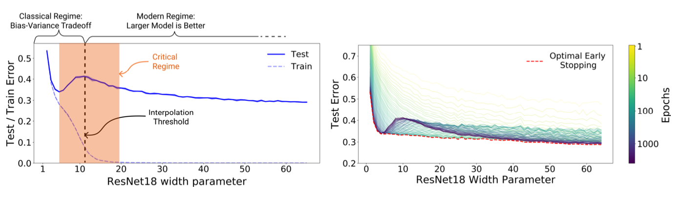
Fig 2. The Double Descent Curve
Because of the two U-shaped curves in the plot of test risk vs model capacity, this phenomenon where the model achieves better generalization as the capacity of the hypothesis class, \(\mathcal{H}\), increases is called the double descent phenomenon.
Why We Created the Testbed
Since double descent is a new phenomenon, there is no central hub where researchers can compare and contrast each other’s results. Researchers Ishaan Gulrajani and David Lopez-Paz from Facebook noticed there was a similar problem in the field of domain generalization. This led them to create DomainBed, a testbed for domain generalization. They implemented seven multi-domain datasets, nine baseline algorithms, and three model selection criteria and are allowing domain generalization researchers to contribute to the testbed.
The goal of this project was to create a similar platform for double descent researchers. DomainBed takes proven algorithms and allows researchers to consistently reproduce results and directly compare algorithms. Given that double descent has been shown to appear in several models with different datasets, creating a testbed that includes these models and datasets would fix a major issue in this research field. Understanding the double descent phenomenon can potentially lead to more robust and accurate machine learning algorithms at no “extra cost”, therefore it is imperative that there is some kind of standardized way to research it.
Project Architecture
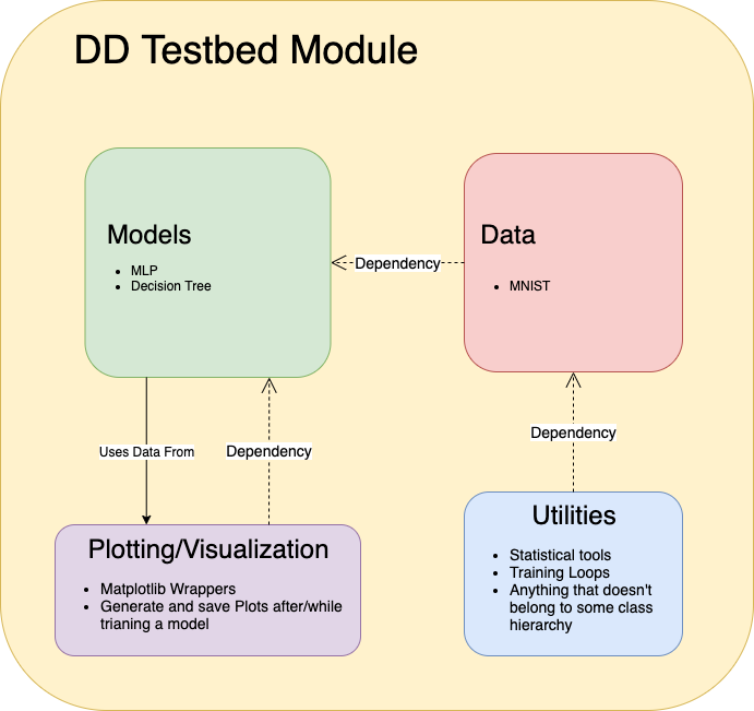
Fig 3. Architecture of the Double Descent Testbed
The testbed has been designed in an object oriented way. This allows users to simply import models from the module, run two or three commands, and have complex experiments running without any boilerplate code. This platform is designed for scientists, though, so users will be given access to the source code and all of the included utilities. This will aid in allowing unique experiments to be conducted using the platform as users can choose the level of abstraction or granularity that they are comfortable with without having to write most of the code themselves.
The project consists of four sub-modules: models, data, utils, and plots. The models sub-module contains abstracted versions of models that have exhibited double descent. At this time, models consists of a fully connected neural network model and a random forest classifier. The data sub-module contains abstracted versions of datasets that have been used in double descent experiments. The models are written in PyTorch or scikit-learn, so the data sub-module is divided into two parts, TorchData and SKLearnData. This allows for more compatibility when a user wants to add a model from either library. The utils sub-module contains any tools that are needed to train models, process data, etc. The main feature of utils is a parameter count generation algorithm that will be discussed later on in the blog post. Lastly, the plots sub-module contains a class with utilities that are specific to plotting, written using Matplotlib. These utilities can be used with the data that is returned by the models after training.
Data
The data module has two versions of the MNIST dataset: a PyTorch implementation and a scikit-learn implementation. The PyTorch implementation contains two PyTorch dataloaders along with exposed parameters such as batch sizes and number of training samples. The PyTorch dataloaders are iterable objects that contain a dataset object within them. By using a dataloader, we can apply transformations to the data and shuffle the dataset prior to training our model. The scikit-learn implementation of MNIST simply returns an \(N \times 784\) matrix where \(N\) is the number of training samples and each row is a 784-dimensional vector that encodes a 28 x 28 image. Both of these implementations download and save the dataset to a local repository where it can be reused without having to wait for the data to be downloaded a second time.
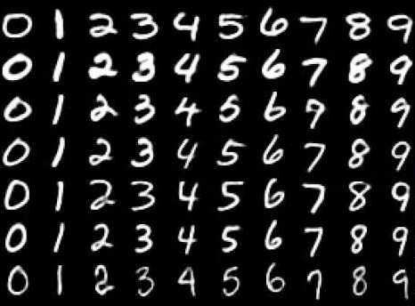
Fig 4. A Sample of Images from the MNIST Dataset
Models
Multilayer Perceptron
The multilayer perceptron is made up of 3 layers, an input layer, a hidden layer, and an output layer (This type of model is sometimes referred to as a two-layer neural network). All three have variable size depending on the dataset that is being trained on. The input layer has \(d = n \cdot m\) units where \(n\) and \(m\) are the dimensions of the input data, as the images are flattened before being passed through the network. The hidden layer has \(h_{i}\) units, where \(h_{i}\) is computed using a desired number of total parameters and the formula for total parameters in Figure 3. The output layer has \(K\) units where \(K\) is the number of output classes. This model also has ReLU activation functions on both the input layer and hidden layer.
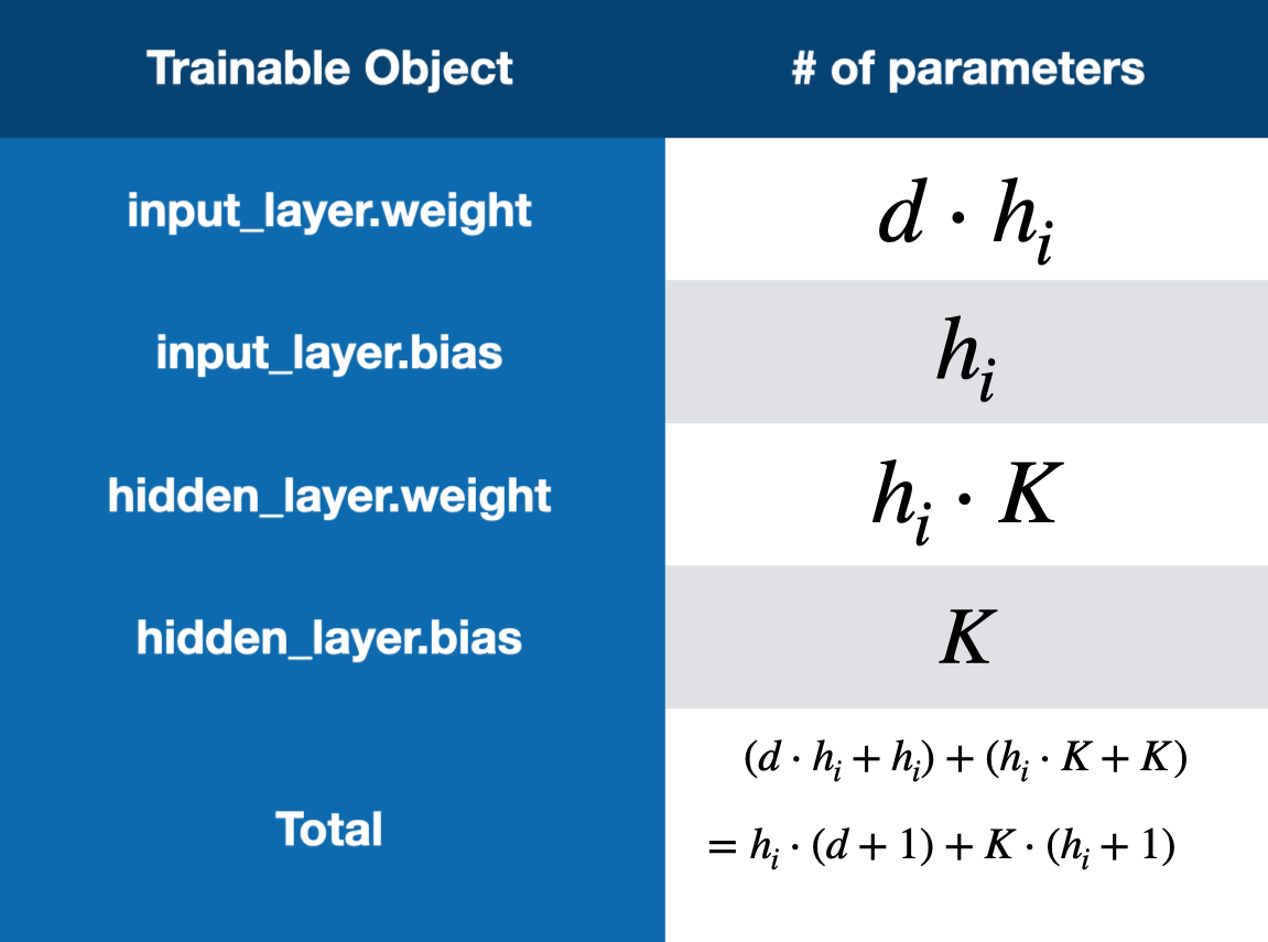
Fig 5. Equation to Calculate Number of Parameters in a Two-Layer Neural Network
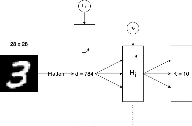
Fig 6. Visualization of our Two-Layer Neural Network
One main feature of the multilayer perceptron wrapper is its built-in TensorBoard functionality. TensorBoard is a visualization dashboard for machine learning experiments. It runs in a web server and reads from a log directory that is produced by the neural network training loop in the double descent testbed. Throughout the training process, we log all training and testing losses for each individual model, as well as the final losses of each model. On this dashboard, we also expose the architecture of the current model that is being experimented on (i.e. its computational graph) and a sample of the dataset that is being used to train the model.
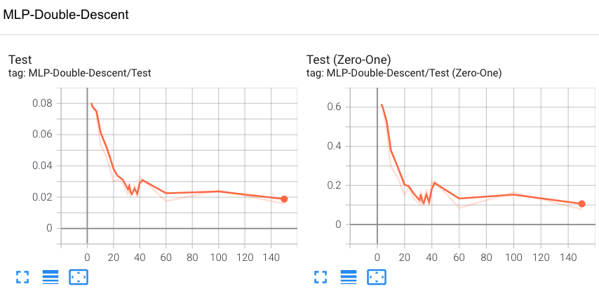
Fig 7. A Screenshot of Tensorboard (Test Loss vs. Model Capacity in # parameters)
Random Forest
The random forest classifier wrapper follows suit by exposing certain features and parameters, such as the maximum number of leaf nodes, the number of trees, and the criterion, to the user when they create an instance of it. Unlike the multilayer perceptron wrapper, which is implemented in PyTorch, the random forest wrapper is implemented in scikit-learn. This means that there is no GPU support, and we cannot take advantage of built-in PyTorch dataloaders. This is not an issue that needs immediate attention, though, as these classifiers only took about half a minute to train in our experiments. Unifying all models under the PyTorch umbrella will be a main area of future work on this testbed.
Utils
Parameter Count Generation Algorithm
When designing the neural network wrapper, we noticed that each of the models took a while to train. Even though the individual models are quite small, when training several of them sequentially for a large number of epochs, single experiments could take several days. To help reduce the time that it takes to run experiments, we developed a parameter count generation algorithm to intelligently choose the next model to train using the number of parameters in the previous model and the final test loss that the model produced. This allowed us to avoid iterating through model capacities (i.e numbers of parameters in the model) at a fixed, constant value. The algorithm was designed to have the highest resolution around the area where models interpolate, or overfit, the data, as this is where the double descent curve is supposed to exhibit itself. We do this by assuming that the double descent curve should look roughly like a \(3^{rd}\) degree polynomial, fitting a \(3^{rd}\) degree polynomial to the model capacity vs. test loss graph, and examining the first derivative of the polynomial that was fit to the data. Algorithm 1 shows the pseudocode for this parameter count generation algorithm.
The algorithm takes a list of previous parameter counts, a list of previous test losses, a flag to determine if the interpolation threshold has been reached, and a tuning parameter \(\alpha\) as input
def Parameter_Count_Generation(param_counts, test_losses, past_interpolation_threshold, alpha):

    current_count = param_counts[-1] # Take last element of param_counts

    # Weight more recent parameter counts more heavily
    weight_vector = [1/n, ... 1/2, 1] # where n = len(param_counts)

    poly = fit_polynomial(param_counts, losses, w)

    # Examine the first derivative of the polynomial
    dy = dy_poly(current_count + eps)

    if dy < 0:
        sgn = 1
    else:
        sgn = 0
        past_interpolation_threshold = True

    next_count = sgn*max(alpha * dy, 3) + 1

    if sgn and past_interpolation_threshold:
        return ceil(next_count) + current_count + 10, past_interpolation_threshold
    else
        return ceil(next_count) + current_count, past_interpolation_threshold

Fig 8. Our Parameter Counts Generation Algorithm Running on a Synthetic Double Descent Curve
Double Descent Training Loop
Each of the models in the testbed has an associated double_descent method that performs the same training procedure for a model over several different capacities. In general, the double_descent method loops over a chosen list of parameter counts for a model (or generates them in an online fashion using the parameter count generation algorithm) and trains the model to any completion criterion that the user has chosen. At the end of each training procedure, final train losses, final test losses, and parameter counts for models of different capacities are aggregated and output to a dictionary of arrays that can be used for visualization or analysis. In the case of the MultilayerPerceptron class, this method contains TensorBoard functionality. To speed up convergence on the multilayer perceptron model, we can toggle a reuse_weights flag to use the weights from the previous model as an initialization for the next model.
If there is a pre-spectified list of parameters, the double descent training loop is the following:
for i in range(len(param_counts)):

    current_index = i

    current_parameter_count = parameter_counts[current_index]

    # Creates new model with specified number of parameters
    reinitialize_model(current_parameter_count)

    losses = train_model()

    # Log losses into TensorBoard or arrays
If the user wants to generate the parameter counts, after a single iteration of training (above), the double descent training loop is the following:
if generate_parameters_enabled:

    steps_past_dd = 0

    past_interpolation_threshold = False

    while steps_past_dd < 4:

        next_count, past_interpolation_threshold = Parameter_Count_Generation(parameter_counts, test_losses)

        parameter_counts.append(next_count)

        current_parameter_counts = parameter_counts[current_index]

        reinitialize_model(current_parameter_count)

        losses = train_model()

        # Log losses into TensorBoard or arrays

        current_index += 1

        if past_interpolation_threshold:
            steps_past_dd += 1